Functions for radial parameterization

e3nn_jax.soft_one_hot_linspace(input: Array, *, start: float, end: float, number: int, basis: str = None, cutoff: bool = None, start_zero: bool = None, end_zero: bool = None)

Projection on a basis of functions.

Returns a set of \(\{y_i(x)\}_{i=1}^N\),

\[y_i(x) = \frac{1}{Z} f_i(x)\]

where \(x\) is the input and \(f_i\) is the ith basis function. \(Z\) is a constant defined such that,

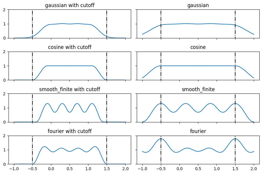
\[\langle \sum_{i=1}^N y_i(x)^2 \rangle_x \approx 1\]

See the last plot below.

Parameters:

• input (jax.Array) – input of shape [...]

• start (float) – minimum value span by the basis

• end (float) – maximum value span by the basis

• number (int) – number of basis functions \(N\)

• basis (str) – type of basis functions, one of gaussian, cosine, smooth_finite, fourier

• cutoff (bool) – if True, the basis functions are cutoff at the start and end of the interval

• start_zero (bool) – if True, the first basis function is zero at the start of the interval

• end_zero (bool) – if True, the last basis function is zero at the end of the interval

Returns:

basis functions of shape [..., number]

Return type:

jax.Array

Examples

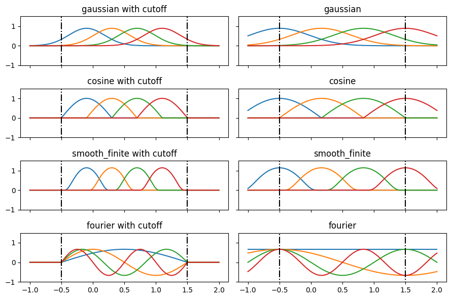
bases = ["gaussian", "cosine", "smooth_finite", "fourier"]
x = np.linspace(-1.0, 2.0, 200)

fig, axss = plt.subplots(len(bases), 2, figsize=(9, 6), sharex=True, sharey=True)

for axs, b in zip(axss, bases):
    for ax, c in zip(axs, [True, False]):
        y = e3nn.soft_one_hot_linspace(x, start=-0.5, end=1.5, number=4, basis=b, cutoff=c)

        plt.sca(ax)
        plt.plot(x, y)
        plt.plot([-0.5]*2, [-2, 2], "k-.")
        plt.plot([1.5]*2, [-2, 2], "k-.")
        plt.title(f"{b}" + (" with cutoff" if c else ""))

plt.ylim(-1, 1.5)
plt.tight_layout()

fig, axss = plt.subplots(len(bases), 2, figsize=(9, 6), sharex=True, sharey=True)

for axs, b in zip(axss, bases):
    for ax, c in zip(axs, [True, False]):
        y = e3nn.soft_one_hot_linspace(x, start=-0.5, end=1.5, number=4, basis=b, cutoff=c)

        plt.sca(ax)
        plt.plot(x, np.sum(y**2, axis=-1))
        plt.plot([-0.5]*2, [-2, 2], "k-.")
        plt.plot([1.5]*2, [-2, 2], "k-.")
        plt.title(f"{b}" + (" with cutoff" if c else ""))

plt.ylim(0, 2)
plt.tight_layout()

e3nn_jax.bessel(x: Array, n: int, x_max: float = 1.0) → Array

Bessel basis functions.

They obey the following normalization:

\[\int_0^c r^2 B_n(r, c) B_m(r, c) dr = \delta_{nm}\]

Parameters:

• x (jax.Array) – input of shape [...]

• n (int) – number of basis functions

• x_max (float) – maximum value of the input

Returns:

basis functions of shape [..., n]

Return type:

jax.Array

Klicpera, J.; Groß, J.; Günnemann, S. Directional Message Passing for Molecular Graphs; ICLR 2020. Equation (7)

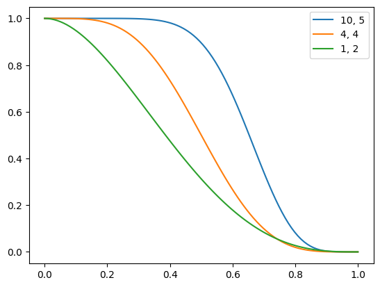
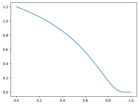
e3nn_jax.poly_envelope(n0: int, n1: int, x_max: float = 1.0) → Callable[[float], float]

Polynomial envelope function with n0 and n1 derivatives euqal to 0 at x=0 and x=1 respectively.

Small documentation available at https://mariogeiger.ch/polynomial_envelope_for_gnn.pdf. This is a generalization of \(u_p(x)\), it is equivalent to \(u_p(x)\) when n0 = p-1 and n1 = 2.

x = jnp.linspace(0.0, 1.0, 100)
plt.plot(x, e3nn.poly_envelope(10, 5)(x), label="10, 5")
plt.plot(x, e3nn.poly_envelope(4, 4)(x), label="4, 4")
plt.plot(x, e3nn.poly_envelope(1, 2)(x), label="1, 2")
plt.legend()

<matplotlib.legend.Legend at 0x7fe72d76f690>

Parameters:

• n0 (int) – number of derivatives equal to 0 at x=0

• n1 (int) – number of derivatives equal to 0 at x=1

• x_max (float) – maximum value of the input, instead of 1

Returns:

polynomial envelope function

Return type:

callable

e3nn_jax.soft_envelope(x: Array, x_max: float = 1.0, arg_multiplicator: float = 2.0, value_at_origin: float = 1.2) → Array

Smooth envelope function.

x = jnp.linspace(0.0, 1.0, 100)
plt.plot(x, e3nn.soft_envelope(x))

[<matplotlib.lines.Line2D at 0x7fe72428b750>]

Parameters:

• x (jax.Array) – input of shape [...]

• x_max (float) – cutoff value

Returns:

smooth (\(C^\infty\)) envelope function of shape [...]

Return type:

jax.Array