Tutorial: learn crystal energies with Nequip
The goal of this tutorial is to show how to use Nequip to train a neural network to predict the energy of crystals.
What this tutorial will cover (and not cover)
jraph to deal with graphsflax to create parameterized modelsoptax to optimize the parametersjraph.pad_with_graphsImport the libraries
For this tutorial we will need the following libraries:
import flax  # neural network modules for jax
import jax
import jax.numpy as jnp
import jraph  # graph neural networks in jax
import matplotlib.pyplot as plt
import numpy as np
import optax  # optimizers for jax
from matscipy.neighbours import neighbour_list  # fast neighbour list implementation

from nequip_jax import NEQUIPLayerFlax  # e3nn implementation of NEQUIP
import e3nn_jax as e3nn
If you want to use a GPU, checkout the jax installation guide.
Here are the pip commands to install everything:
pip install -U pip
pip install -U "jax[cpu]"

pip install -U flax jraph optax
pip install -U matscipy
pip install -U matplotlib
pip install -U e3nn_jax

pip install git+https://github.com/mariogeiger/nequip-jax
Dataset
Let’s create a very simple dataset of few crystals from materials project made only of carbon atoms. Materials project provides a Predicted Formation Energy for each crystal, and we will use this as our target.
To compute the graph connectivity we use matscipy library which has a very fast neighbour list implementation.
def compute_edges(positions, cell, cutoff):
    """Compute edges of the graph from positions and cell."""
    receivers, senders, senders_unit_shifts = neighbour_list(
        quantities="ijS",
        pbc=np.array([True, True, True]),
        cell=cell,
        positions=positions,
        cutoff=cutoff,
    )

    num_edges = senders.shape[0]
    assert senders.shape == (num_edges,)
    assert receivers.shape == (num_edges,)
    assert senders_unit_shifts.shape == (num_edges, 3)
    return senders, receivers, senders_unit_shifts
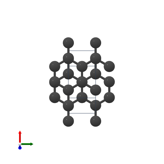
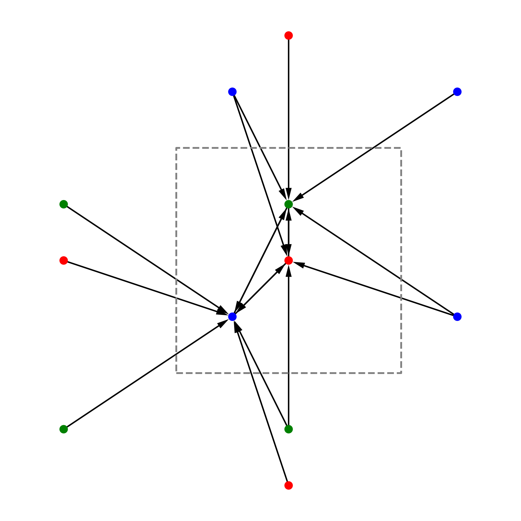
This image shows the edges created by matscipy.neighbours.neighbour_list for an example crystal in 2D. Note that all the edges point (receivers side) to an atom in the central cell.
Then we use jraph to create a graph objects and (later) batch them together. jraph is a library for graph neural networks in jax developed by DeepMind.
The following function create_graph creates a graph object from the given positions, cell and energy of the crystal.
Each crystal is stored in a jraph.GraphsTuple, which is the cornerstone datatype of the jraph library. It is a named tuple that contains all the information about a graph. The documentation of jraph.GraphsTuple can be found here.
def create_graph(positions, cell, energy, cutoff):
    """Create a graph from positions, cell, and energy."""
    senders, receivers, senders_unit_shifts = compute_edges(positions, cell, cutoff)

    # In a jraph.GraphsTuple object, nodes, edges, and globals can be any
    # pytree. We will use dicts of arrays.
    # What matters is that the first axis of each array has length equal to
    # the number of nodes, edges, or graphs.
    num_nodes = positions.shape[0]
    num_edges = senders.shape[0]

    graph = jraph.GraphsTuple(
        # positions are per-node features:
        nodes=dict(positions=positions),
        # Unit shifts are per-edge features:
        edges=dict(shifts=senders_unit_shifts),
        # energy and cell are per-graph features:
        globals=dict(energies=np.array([energy]), cells=cell[None, :, :]),
        # The rest of the fields describe the connectivity and size of the graph.
        senders=senders,
        receivers=receivers,
        n_node=np.array([num_nodes]),
        n_edge=np.array([num_edges]),
    )
    return graph
We need to specify the cutoff for the neighbour list. This is the distance up to which we consider two atoms to be connected. All the distances here are in angstroms.
cutoff = 2.0 # in angstroms
Now we can create the graphs for the crystals. The values of the positions, cell and energy are taken from the materials project website.
mp47 = create_graph(
    positions=np.array(
        [
            [-0.0, 1.44528, 0.26183],
            [1.25165, 0.72264, 2.34632],
            [1.25165, 0.72264, 3.90714],
            [-0.0, 1.44528, 1.82265],
        ]
    ),
    cell=np.array([[2.5033, 0.0, 0.0], [-1.25165, 2.16792, 0.0], [0.0, 0.0, 4.16897]]),
    energy=0.163,  # eV/atom
    cutoff=cutoff,
)
print(f"mp47 has {mp47.n_node} nodes and {mp47.n_edge} edges")

mp48 = create_graph(
    positions=np.array(
        [
            [0.0, 0.0, 1.95077],
            [0.0, 0.0, 5.8523],
            [-0.0, 1.42449, 1.95077],
            [1.23365, 0.71225, 5.8523],
        ]
    ),
    cell=np.array([[2.46729, 0.0, 0.0], [-1.23365, 2.13674, 0.0], [0.0, 0.0, 7.80307]]),
    energy=0.008,  # eV/atom
    cutoff=cutoff,
)
print(f"mp48 has {mp48.n_node} nodes and {mp48.n_edge} edges")

mp66 = create_graph(
    positions=np.array(
        [
            [0.0, 0.0, 1.78037],
            [0.89019, 0.89019, 2.67056],
            [0.0, 1.78037, 0.0],
            [0.89019, 2.67056, 0.89019],
            [1.78037, 0.0, 0.0],
            [2.67056, 0.89019, 0.89019],
            [1.78037, 1.78037, 1.78037],
            [2.67056, 2.67056, 2.67056],
        ]
    ),
    cell=np.array([[3.56075, 0.0, 0.0], [0.0, 3.56075, 0.0], [0.0, 0.0, 3.56075]]),
    energy=0.138,  # eV/atom
    cutoff=cutoff,
)
print(f"mp66 has {mp66.n_node} nodes and {mp66.n_edge} edges")

mp169 = create_graph(
    positions=np.array(
        [
            [-0.66993, 0.0, 3.5025],
            [3.5455, 0.0, 0.00033],
            [1.45739, 1.22828, 3.5025],
            [1.41818, 1.22828, 0.00033],
        ]
    ),
    cell=np.array([[4.25464, 0.0, 0.0], [0.0, 2.45656, 0.0], [-1.37907, 0.0, 3.50283]]),
    energy=0.003,  # eV/atom
    cutoff=cutoff,
)
print(f"mp169 has {mp169.n_node} nodes and {mp169.n_edge} edges")
mp47 has [4] nodes and [16] edges
mp48 has [4] nodes and [12] edges
mp66 has [8] nodes and [32] edges
mp169 has [4] nodes and [12] edges
Now that we have mp47, mp48, mp66 and mp169 as graphs, we can batch them together to create a dataset. Batching is an important concept in jraph, it merges different graphs into a single graph. The batch function takes a list of graphs and returns a single graph with the same fields as the input graphs. The n_node and n_edge fields are used to keep track of the number of nodes and edges in each graph.
dataset = jraph.batch([mp47, mp48, mp66, mp169])
print(f"dataset has {dataset.n_node} nodes and {dataset.n_edge} edges")

# Print the shapes of the fields of the dataset.
print(jax.tree_util.tree_map(jnp.shape, dataset))
dataset has [4 4 8 4] nodes and [16 12 32 12] edges
GraphsTuple(nodes={'positions': (20, 3)}, edges={'shifts': (72, 3)}, receivers=(72,), senders=(72,), globals={'cells': (4, 3, 3), 'energies': (4,)}, n_node=(4,), n_edge=(4,))
Model
Before defining the model, we need to make sure we properly take into account the periodic boundary conditions of the crystals. The model will need to know the relative vectors between the atoms in the crystal. We know the positions of the atoms inside the unit cell, but we need to know the relative vectors between the atoms even if they don’t belong to the same cell.
def get_relative_vectors(senders, receivers, n_edge, positions, cells, shifts):
    """Compute the relative vectors between the senders and receivers."""
    num_nodes = positions.shape[0]
    num_edges = senders.shape[0]
    num_graphs = n_edge.shape[0]

    assert positions.shape == (num_nodes, 3)
    assert cells.shape == (num_graphs, 3, 3)
    assert senders.shape == (num_edges,)
    assert receivers.shape == (num_edges,)
    assert shifts.shape == (num_edges, 3)

    # We need to repeat the cells for each edge.
    cells = jnp.repeat(cells, n_edge, axis=0, total_repeat_length=num_edges)

    # Compute the two ends of each edge.
    positions_receivers = positions[receivers]
    positions_senders = positions[senders] + jnp.einsum("ei,eij->ej", shifts, cells)

    vectors = e3nn.IrrepsArray("1o", positions_receivers - positions_senders)
    return vectors
Now we define the model layer based on Nequip architecture.
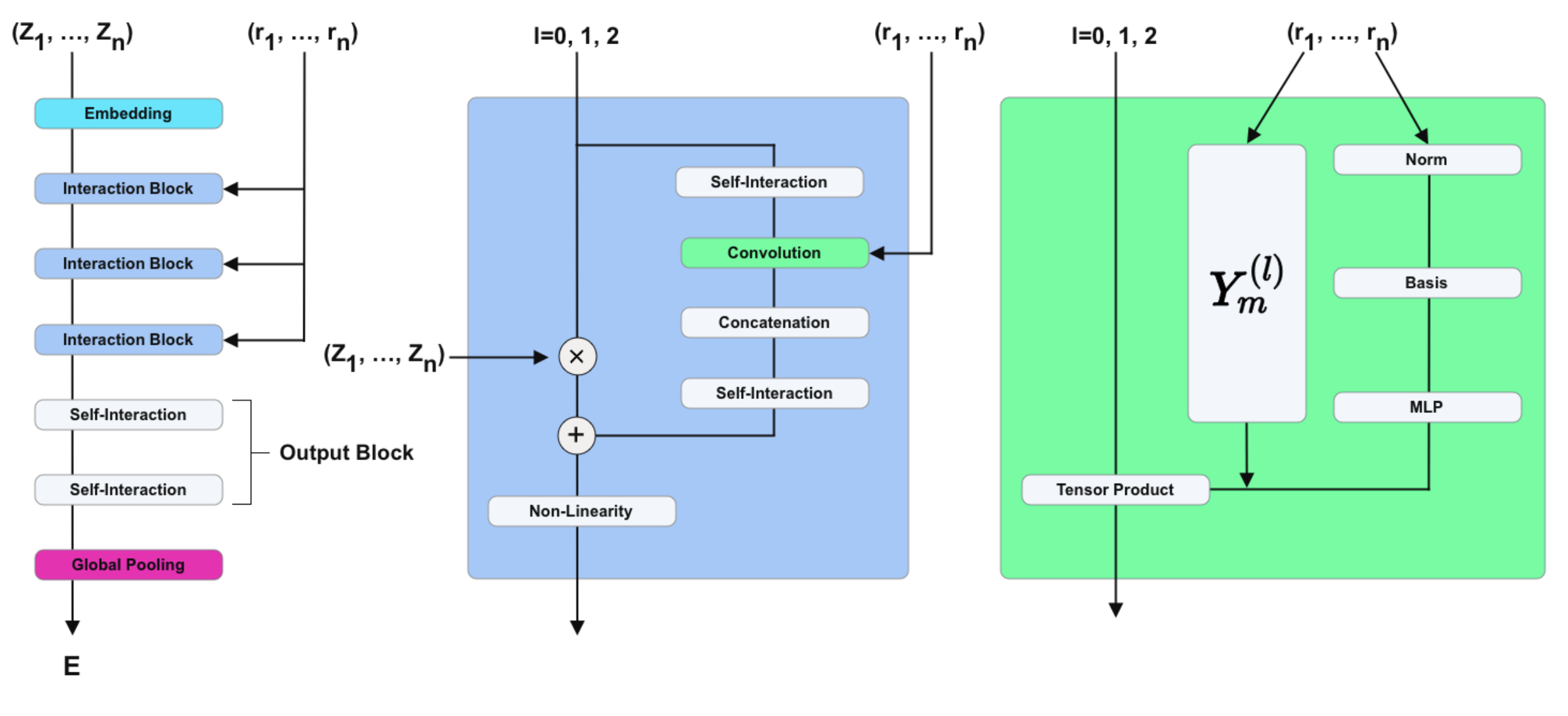
For that we will use the implementation available at github.com/mariogeiger/nequip-jax.
This implementation provides a NEQUIPLayerFlax class that implements the Interaction Block part of the Nequip architecture (the blue box in the figure above).
The Embedding, Self-Interaction and Global Pooling parts of the Nequip architecture are not implemented in nequip-jax and we will need to implement them ourselves below.
The class below defines a flax-Module. flax is a neural network library that is built on top of jax. flax provides a Module class that is similar to nn.Module in PyTorch. flax also provides a compact decorator that allows us to define the __call__ method of the Module in a more concise way. See the flax documentation for more details.
class Model(flax.linen.Module):
    @flax.linen.compact
    def __call__(self, graphs):
        num_nodes = graphs.nodes["positions"].shape[0]
        senders = graphs.senders
        receivers = graphs.receivers

        vectors = get_relative_vectors(
            senders,
            receivers,
            graphs.n_edge,
            positions=graphs.nodes["positions"],
            cells=graphs.globals["cells"],
            shifts=graphs.edges["shifts"],
        )

        # We divide the relative vectors by the cutoff
        # because NEQUIPLayerFlax assumes a cutoff of 1.0
        vectors = vectors / cutoff

        # Embedding: since we have a single atom type, we don't need embedding
        # The node features are just ones and the species indices are all zeros
        features = e3nn.IrrepsArray("0e", jnp.ones((num_nodes, 1)))
        species = jnp.zeros((num_nodes,), dtype=jnp.int32)

        # Apply 3 Nequip layers with different internal representations
        for irreps in [
            "32x0e + 8x1o + 8x2e",
            "32x0e + 8x1o + 8x2e",
            "32x0e",
        ]:
            layer = NEQUIPLayerFlax(
                avg_num_neighbors=20.0,  # average number of neighbors to normalize by
                output_irreps=irreps,
            )
            features = layer(vectors, features, species, senders, receivers)

        # Self-Interaction layers
        features = e3nn.flax.Linear("16x0e")(features)
        features = e3nn.flax.Linear("0e")(features)

        # Global Pooling
        # Average the features (energy prediction) over the nodes of each graph
        return e3nn.scatter_sum(features, nel=graphs.n_node) / graphs.n_node[:, None]
Training
Now that we defined the model, we need to define the loss function to train it. For this example we will use the mean squared error.
def loss_fn(preds, targets):
    assert preds.shape == targets.shape
    return jnp.mean(jnp.square(preds - targets))
Now let’s use the magic of flax to initialize the model and use the magic of optax to define the optimizer and initialize it as well.
As optimizer we will use Adam. This optimizer needs to keep track of the average of the gradients and the average of the squared gradients. This is why it has a state. The state is initialized with opt.init.
random_key = jax.random.PRNGKey(0)  # change it to get different initializations

# Initialize the model
model = Model()
params = jax.jit(model.init)(random_key, dataset)

# Initialize the optimizer
opt = optax.adam(1e-3)
opt_state = opt.init(params)
Let’s define the training step. We will use jax.jit to compile the function and make it faster.
This function takes as input the model parameters, the optimizer state and the dataset and returns the updated optimizer state, the updated model parameters and the loss.
@jax.jit
def train_step(opt_state, params, dataset):
    """Perform a single training step."""
    num_graphs = dataset.n_node.shape[0]

    # Compute the loss as a function of the parameters
    def fun(w):
        preds = model.apply(w, dataset).array.squeeze(1)
        targets = dataset.globals["energies"]

        assert preds.shape == (num_graphs,)
        assert targets.shape == (num_graphs,)
        return loss_fn(preds, targets)

    # And take its gradient
    loss, grad = jax.value_and_grad(fun)(params)

    # Update the parameters and the optimizer state
    updates, opt_state = opt.update(grad, opt_state)
    params = optax.apply_updates(params, updates)

    return opt_state, params, loss
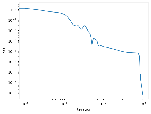
Finally, let’s train the model for 1000 iterations.
losses = []
for _ in range(1000):
    opt_state, params, loss = train_step(opt_state, params, dataset)
    losses.append(loss)
Did it work?
plt.plot(losses)
plt.xscale("log")
plt.yscale("log")
plt.xlabel("Iteration")
plt.ylabel("Loss")
Text(0, 0.5, 'Loss')